AC209a Data Science

Overview

Motivation

Exchange rates are important indicators of real and perceived economic performance. Fluctuations in a country's exchange rate directly reflect changes in economic confidence, a fact that became particularly salient during the recent global financial crisis and Brexit referendum. Furthermore, as foreign currencies are one of the most liquid assets traded in global financial markets, any relevant news or development about a country's economy is very quickly priced into exchange rates, and a belief in the strong efficient markets hypothesis would lead one to believe that exchange rates are not only very difficult to predict, but potentially impossible to predict in practice.

Objectives

In this project, we aim to predict future exchange rates at a weekly level. We apply techniques from time series analysis and natural language processing to identify trends in the exchange rate for prediction. We hypothesise that changes in business news sentiment can be used to predict movements in the exchange rate, leading to more accurate predictors when combined with predictors from time series analysis. Our goal is to build a time series prediction model that incorporates sentiment scores of news articles. We decided to focus on business news as we postulate that news in this segment is most closely related to and affected by exchange rates. Other news segments we considered were politics and world news, however we decided to focus initally on business related news. Through this project we sought to answer a few key questions:

How accurately can next week's exchange rate be predicted using only past values of exchange rate? What form would such a time series predictive model take?
Can a sentiment "signal" be extracted from news articles over a period of time and what would this signal look like?
Can the sentiment signal be incorporated into the time series predictive model, and if so does it improve the predictive accuracy of the model?

Approach

We began our study by collecting UK/US exchange rate data and business news articles in the period 2010-2016. The subsequent analysis involved two components. The first was a univariate time series predictive model of the exchange rate data. The second was a sentiment analysis algorithm to determine the weekly business sentiment score. The results of this analyis formed the creation of a multivariate time series model incorporating sentiment scores. The predictive accuracies of the models were compared the models were used to generate a one week forecast of the exchange rate.

Sentiment Analysis

Sentiment analysis of news articles was performed using SentiWordNet, a public dictionary of words with sentiment scores, which has been trained via semi-supervised learning.

SentiWordNet Methodology

1. Selection of Relevant Articles

From all the scraped articles, we first filtered based on relevance to economic health. This involved building a set of words and phrases based in economic theory to indicate relevance. The article were searched to test for the occurence of any of the words from the relevant set. An article was considered relevant if the number of terms matched in the relevance set was above a certain threshold. We visualised the average number of relevant articles weekly under different relevance thresholds (where a higher threshold results in a lower number of articles). After considering different values, we determined the optimal threshold to be 3 words. This was decided by ensuring that a sufficient number of articles were classed as relevant weekly in order to generate weekly sentiment scores (such that no week had zero relevant articles), whilst also ensuring an excessive number of irrelevant articles were excluded.

Of the relevant business articles, the most common words can be visualized below

2. Tokenizing

Splitting article body into sentences, then into words

SentinetWordNet provides a trained index of words and their corresponding positive, negative and netural sentiments (where the sum of these sentiments equal 1). To generate sentiments at an article level, the articles were processed into count vectors. Stopwords were stripped and a dictionary of words was built using the entire corpus. The articles were then vectorised (count vectors of words in the dictionary). The mean sentiment of the words in the vector were used as the sentiment score for the entire article. A potential problem behind this method is that we may not obtain accurate sentiments for sections of the article which depend on more sophisticated understanding of the natural language at a phrase or sentence level. However, given the computation time required to use more sophisticated natural language processing techniques (such as Word2Vec or Doc2Vec) and the total number of articles to be considered across the time period, we decided to proceed with the simpler model.

3. Filtering Neutrality

Removing sentences with neutral sentiment from the original article

Given each article, we removed any sentences which had very high neutral sentiment scores. This ensured that our sentiment score generator would only focus on sentences which implied strong sentiment, resolving a previous problem of obtaining very low positive/negative sentiment scores from our model. We also investigated different neutral sentiment thresholds to see which would be the most effective for removing neutral sentiment sentences. For each of these thresholds, we calculated the sentiment scores of the articles (with neutral sentences removed) at a weekly level. This time series of positive and negative sentiment scores was compared with the exchange rate time series to obtain correlation values. We chose the optimal threshold by maximising the magnitude of correlation values. This gave an optimal threshold of 0.9 and all articles were processed using this value to remove neutral sentences

4. Weekly sentiment

Averaging article sentiments at a weekly level to obtain weekly sentiment scores.

Having developed a method to generate sentiment scores for a given article, we simply took the mean average of the articles at a given week to generate the sentiment scores associated to that week. For future work, it may be worth considering potential ways to weight different articles' sentiments based on factors such as their popularity.

5. Smoothing

Reducing the weekly variance of sentiment scores with a rolling average

Having generated weekly sentiment scores, initially the high weekly variance did not allow any visible trends to be noticed. We resolved this by smoothing the weekly sentiment scores using a rolling average of a fixed number of preceeding weeks. This idea has a natural motivation - overall sentiment on a given week is also dependant on the sentiment of the previous few weeks. The optimal number of preceding weeks used to smoothen the sentiment scores was chosen by maximising the correlation between the exchange rate and the sentiment score time series. The smoothed sentiment scores now show visible correlation with the exchange rate, especially during times such as the Brexit referendum. This is shown below.

The weekly scores were saved and used in the multivariate prediction model

View the Code

Time Series Analysis

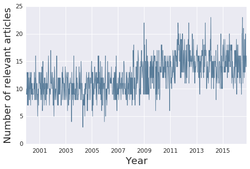
Baseline Model

How well can we predict exchange rates considering only past values?

In building a baseline model we considered several approaches including univariate versions of ARIMA models (autoregreesive integrated moving average models involving using lagged values of the response variable as well as moving average terms), and autoregressive models as well as multivariate models incorporating Libor rates and lastly sentiment scores.

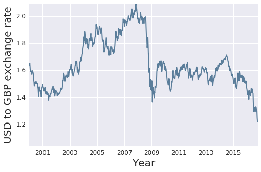
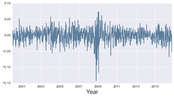
Exchange Rate Series

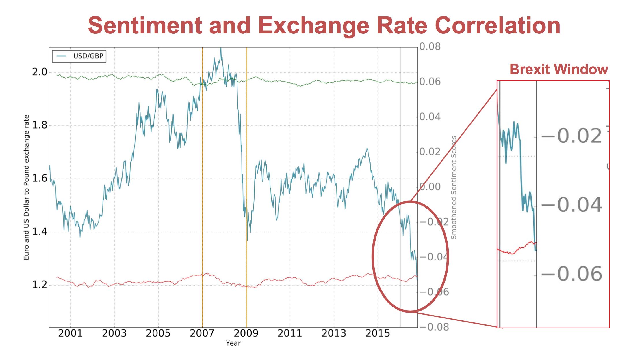
Let's take a look again at the exchange rate plot, zooming in on times of interest

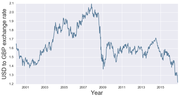
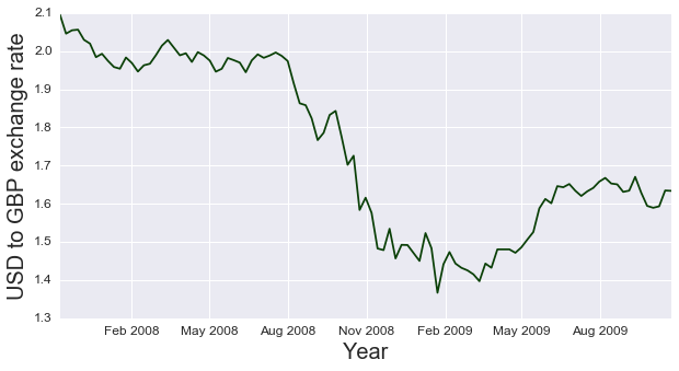
First, lets take a look at the global financial crisis, and event that preciptated a drastic change in the UK-US exchange rate.

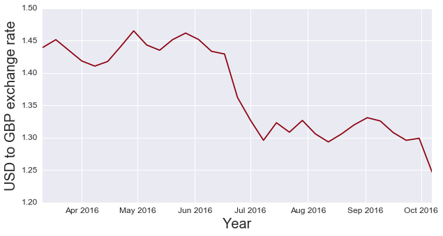
Next, take a look at the at the time period around the Brexit referendum, which saw the value of the GBP at a local minimum relative to a 25 year time horizon.

Stationarity

An important assumption in much of models underlying time series analysis is that the mean and variance of the data do not change over time; if the data has an underlying trend, this will certainly not be true. As such, most time series analysis occurs on data rendered stationary, traditionally by taking first differences. After differencing, we see that aside from a time of extreme variation around the global financial crisis, data is reasonably stationary with mean zero and relatively stable variance outside of the 2008-2010 time frame. Keeping the anomalies of the financial crisis in mind, we can move on to the next segment in building our model.

Autocorrelation

Let's first start by taking a deeper dive into the first lag of the first-differenced exchange rate as this should give us some information as to whether or not a simple AR(1) process can adequately model our data. If we see a non-zero slope in the correlation plot, we can infer that there is, in fact, a good relationship between this week's exchange rate and last week's exchange rate.

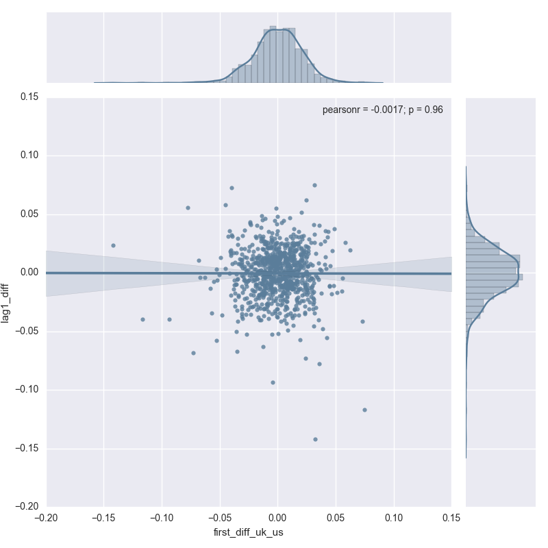
The first difference is almost certainly zero, with both axes having data appearing to be drawn from a roughly normal distribution with mean zero. There does not appear to be much gleaned from relying entirely on the first lag.

Let's now take a look at further lags (lags 2 through 40) to see if there is any other information available in prior lags.

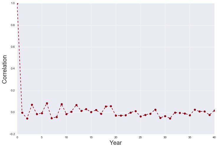
The lags appear to bounce around zero - an AR process might not be able to glean all that much from the underlying data, although regularization might improve this (discussed later)

Univariate ARMA models

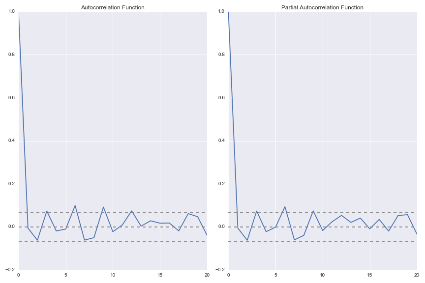
Although we saw from the autocorrelation plot above that an AR processes will likely perform trivially, a well-developed baseline model is required against which we will compare our sentiment score-augmented model.

ARIMA models are set of time series methods that include autoregressive components (AR), differencing (I), and moving average terms (MA) in order to capture various dimensions by which time series trends can be described.

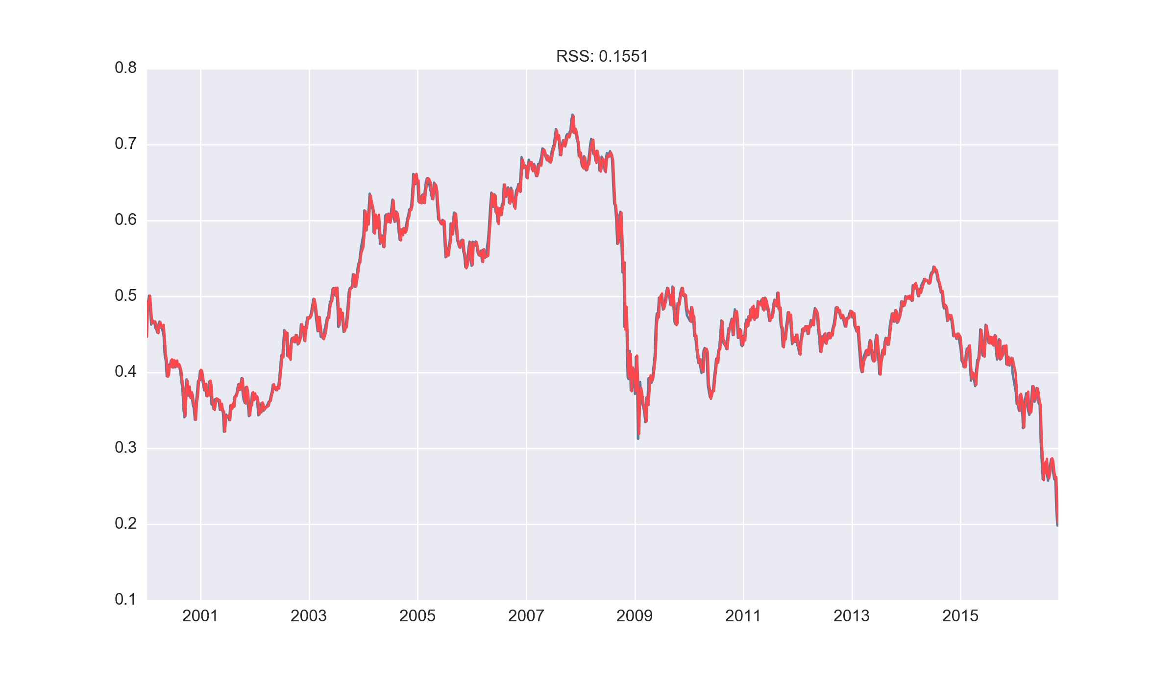
AR model

As mentioned earlier, AR terms capture the number of lags to be used by the model. Here, we select an AR(6) process as the sixth lag is somewhat significant in both the ACF and PACF plots above. The AR(6) process appears to perform quite well (although we should remember that exchange rates do not vary all too much week over week).

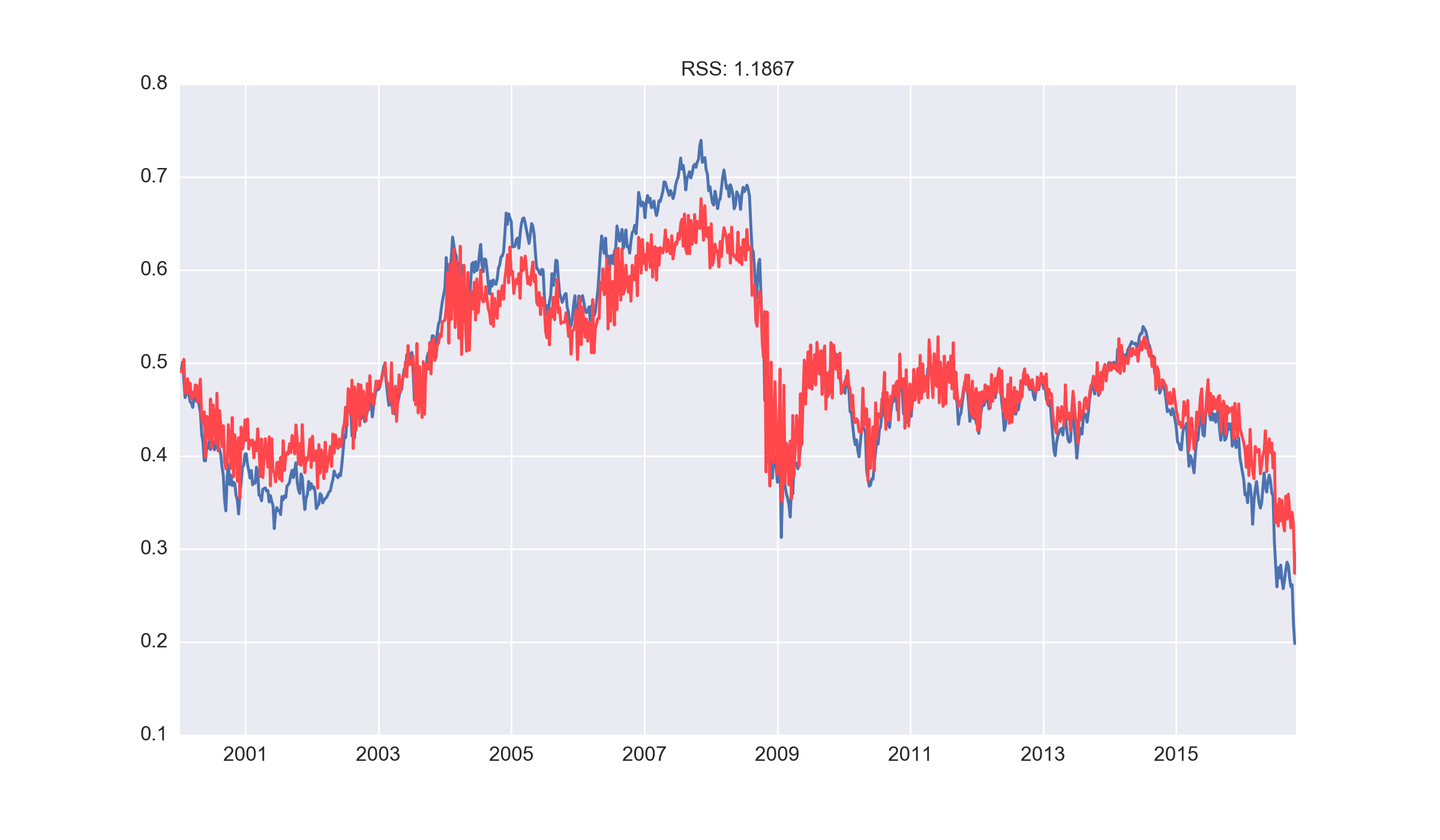
MA model

We also considered a standalone moving average model (using two moving average terms) for the sake of exploration. This appeared to attenuate the magnitude of our predictions and lead to a poor model result.

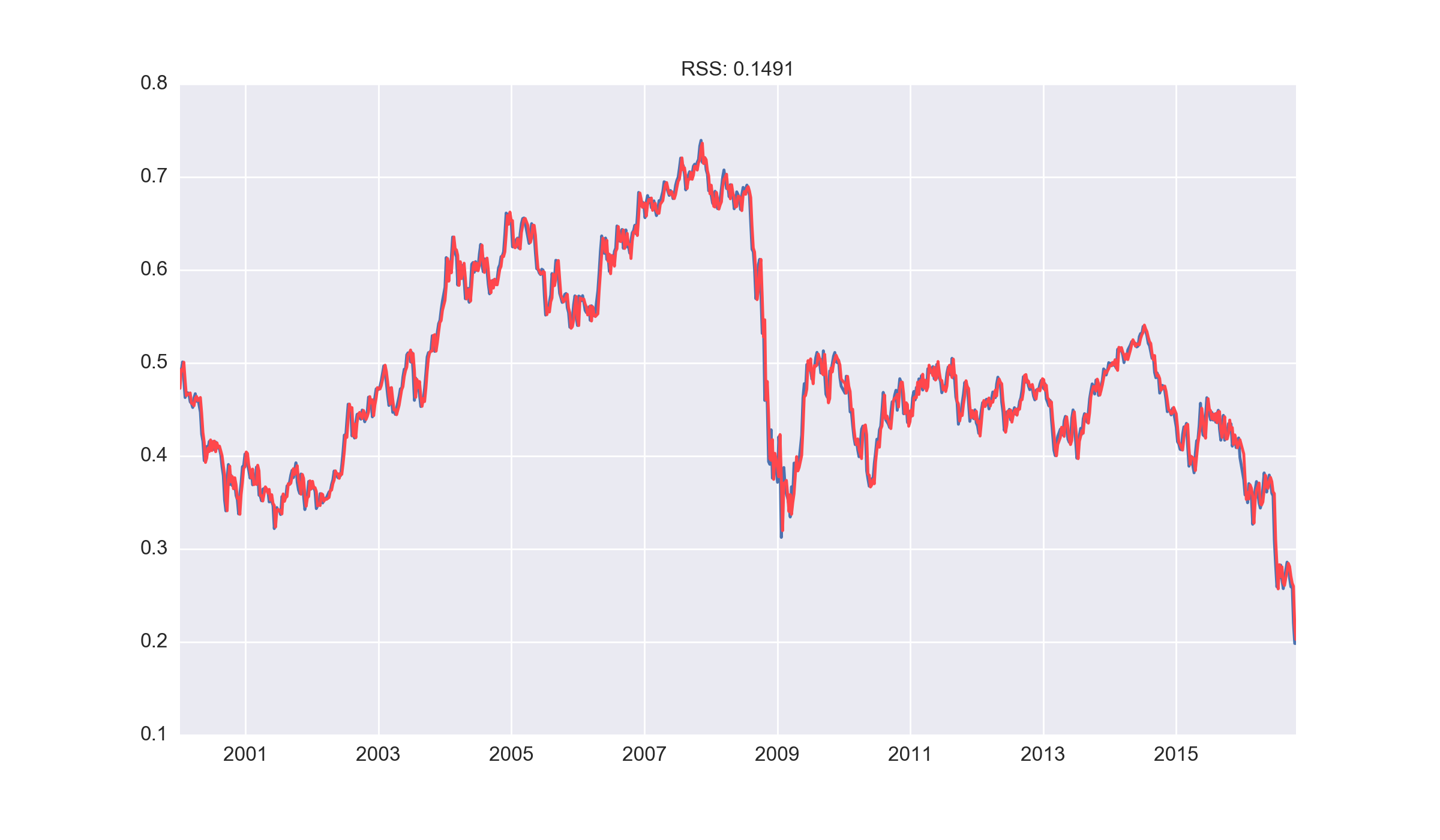
ARMA model

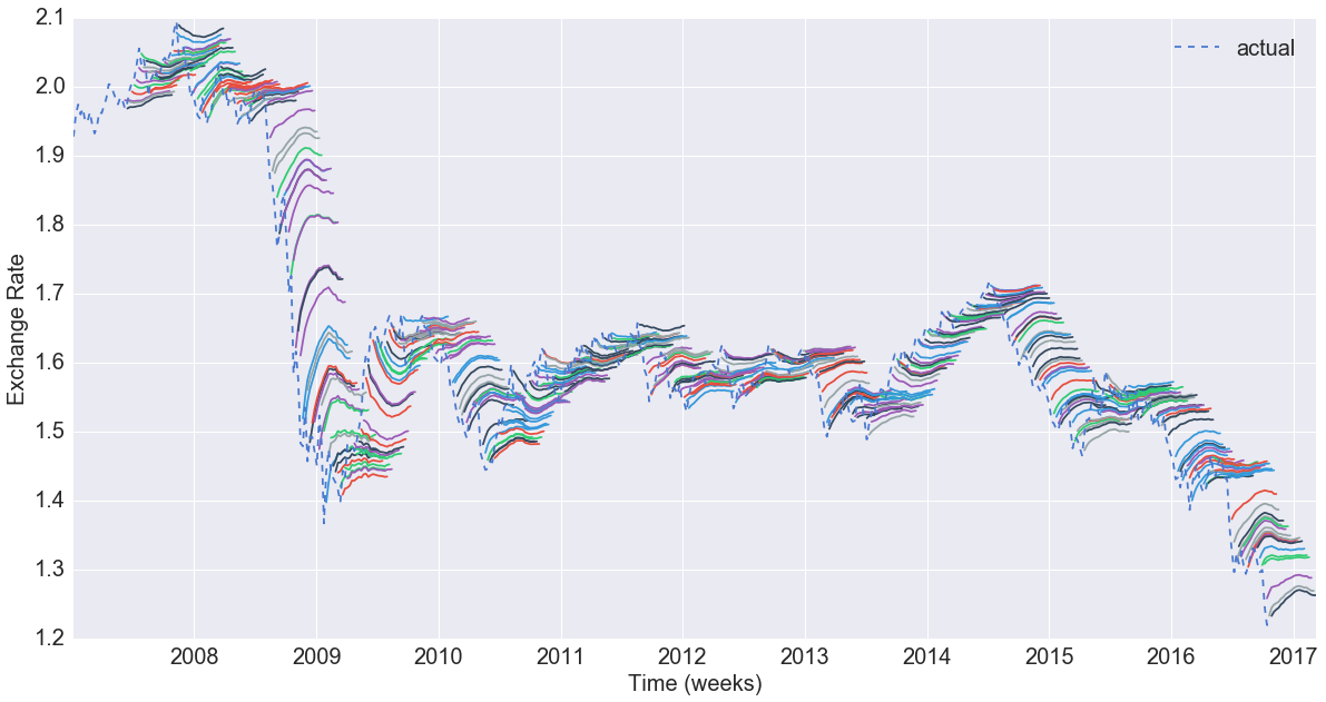
Our final baseline model was a combined ARMA (6,5) process that yielded the lowest RSS on the data, with a plot of the prediction overlayed on the original data below.

Lasso regression model

For further improvements from the baseline model, several other models were considered including regression models with L1 and L2 regularisation. This is equivalent to an autoregressive model and would enable us to examine the magnitude of the coefficients assigned to each lag (i.e. the importance of each lag in generating a prediction).

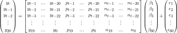
1. Create a matrix of lagged predictors

Matrices of predictors were generated with the lagged response variable and this was used with Lasso regression to determine the coefficients of the lags. The data was of the form:

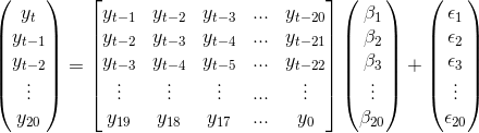
To determine the number of lags used in our model, we split the given data into training and test sets and analysed the cross validation scores. This is gave 20 lags as being the optimal choice, as shown in the matrix above.

2. Split into test and train sets and analyse model forecasts

As the predictors are given by the rows of the predictor matrix, each observation is independent i.e. sequential slices of the data are no longer required for cross validation. The data was randomly split into test (40%) and train (60%) sets

3. Use lasso regression to fit a model to the training data

Having chosen the number of lags, we now fit a lasso regression model on the training data. We choose to use the lasso because it would give sparse coefficients in our prediction lag variables, so that potential interpretations can be made after the fit. Cross validated Lasso regression was used to optimise the hyperparameters.

4a. Visualising the predictions on the test set

We first visualise the predictions from the lasso model on the test set, to obtain a sense of the overall fit compared to the actual valus

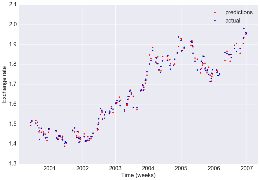
As visualised above, our predictions are close to the actual exchange rates on the test set and the R2 of the model is high (0.987)

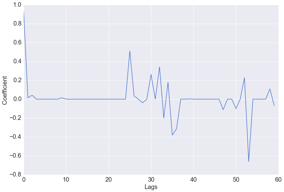
4b. The regression coefficients of the fitted model

We can analyse which of the time lags are the most significant in our model by considering the fitted regression coefficients

Visualisation of the coefficient values shows that beyond the first lag, the subsequent lags have little predictive value. Lasso regression squashes the predictive power of some coefficients in favour of others, and in this case has put all the predictive power in the first lag.

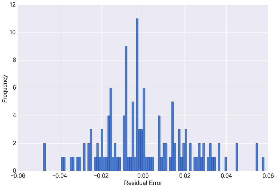
4c. Residual errors of the model

We can analyse the distribution of the residual errors of the model to determine if there is a predictive bias

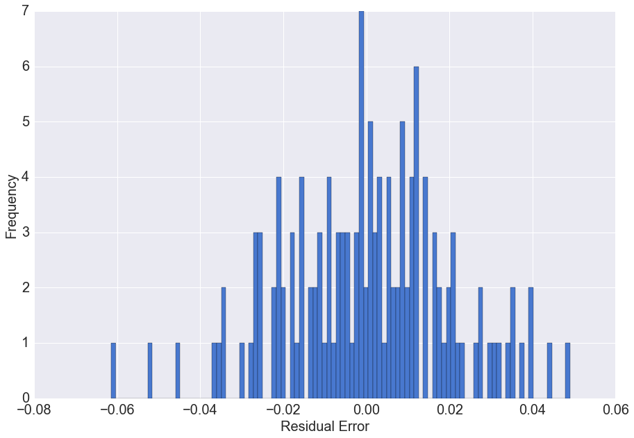
The residual errors have a distribution with mean approximately zero. This means on average our prediction model does not under or overestimate the actual values.

The univariate model is seen to have high predictive accuracy in determining the exchange rate for the following week, however forecasts further in the future are likely to have much lower accuracy (discussed later) and in these situations, the effect of news sentiment may be useful

Multivariate Lasso regression

A predictor matrix containing 20 lags of preceeding exchange rate, 20 lags of preceeding positive sentiment scores, and 20 lags of preceeding negative sentiment scores was constructed of the form

Again we can analyse which of the time lags and the positive/ negative sentiment lags are the most significant in our model, by considering the fitted regression coefficients

The lasso regression model has assigned high positive predictive value to the first lag as before, but the coefficients of lags of the sentiment scores are also seen to have non-zero magnitude. The positive sentiment score approximately 5 weeks prior, as well as the negative sentiment score approximately 3 weeks prior are both seen to have large coefficient values. The coefficients vary for different testing and training sets indicating that the high values for sentiment in certain weeks may be random - i.e. the important lags of sentiment are not the same over time. This will be investigated further in our future work.

Residual errors of the model

We can again analyse the distribution of the residual errors of the model

The residual errors have a distribution with mean approximately zero. This means on average our prediction model does not under or overestimate the actual values.

Model Comparison

Finally, we consider the R^2 values of the different models considered for comparison with our final foreact model which incorporates the sentiment scores.

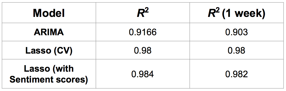
There is little increase in the predictive accuracy of the model with the incorporation of sentiment scores, showing that a simpler univariate model is in fact equally as useful as a more complex model with a larger predictor space

View the Code

Forecasting

The time series lasso model alongside the sentiment scores were used to generate forecasts of the exchange rate for different forecast horizons

Forecast Methodology

Exchange rate forecasts were generated in an incremental process:

1. The lags of time step t were used to generate a prediction for time step t+1

2. This was used as the best estimate of the exchange rate at time t+1 and used as one of the predictors to predict the value of the exchange rate at time t+2

This incremental forecasting process was continued up to the desired forecasting horizon. It is important to note that at each forecasting step, the error increases significantly and the confidence bounds after even 2 time steps forecasts are large. The plot below shows 20 week forecasts generated from each time point. The forecasts are shown as the coloured lines.

The forecasts are seen to have very little predictive accuracy beyond predicting 1-2 weeks in the future. This result is unsurprising. Given the inherent unpredictable nature of exchange rates and their sensitivity to changes in the world, it would be unrealistic to expect that the exchange rate could be forecasted several weeks or months into the future. Looking more closely at the direction of prediction, during the sharp fall in exchange rates during the financial crisis (late 2008), the predictions are in the positive direction, and it takes several months before the direction of prediction aligns with the local direction of movement. Following the financial crisis, the predictions all show the value decreasing from the value at the local time point. This analysis shows that long horizon forecasts of the exchange rate are difficult and most probably inaccurate.

Model Comparison

Considering the R^2 values of the different models for one week forecasts, the ARMA model is seen to have the lowest accuracy. A univariate lasso model is almost equally as good as a model with sentiment scores included suggesting that the sentiment scores provide little additional predictive power.

View the Code

Conclusions

In this project our goal was to predict future exchange rates at a weekly level. Using techniques from time series analysis and SentiWordNet, we developed models for exchange rate prediction which incorporated weekly sentiment scores from relevant news articles. We found that the addition of sentiment scores into the model does not necessarily result in an improvement in prediction accuracy, contrary to our initial hypothesis.

This is actually consistent with existing research literature (see [3]), where it is found that news sentiments are useful in indicating the direction of exchange rate movements but ineffective in predicting the magnitude of the exchange rate movements. Therefore, incorporating the sentiment scores through a large predictor space does not necessarily lead to improved predictive accuracy.

This project has highlighted the intrinsic difficulties of predicting exchange rates using news sentiments. As the exchange rate market is so liquid and fast-paced, any impact from extraneous events is reflected immediately on the rates, often much sooner than when an article is written about these events. Perhaps for future work it may be more fruitful to consider sentiment of news sources such as Twitter where news is reported much faster.

Future Work

There are various areas we can investigate to further improve our model and develop this project:

Differencing the exchange rate time series data in forming the predictor matrix
Adding differenced sentiment scores, under the hypothesis that changes in the sentiment could rive changes in the exchange rate rather than absolute values
Elastic net regularisation using the matrix of lagged predictors (a combination of L1 and L2 regularisation)
Vector autoregressive models
Investigate more sophisticated models such as AFIRMA which are commonly used for forecasting high frequency time series data
Incorporate sentiment scores from a wider range of news sources outside the Guardian
Investigate more sophisticated natural language processing techniques such as Word2Vec or Doc2Vec which can consider articles at a sentence level rather than a word level

Overview

Data Collection and Exploration

Economic and News data was collected over a 16 year period from 2010-2016 and cleaned to provide weekly data

Economic Indicator Data

News Data

Sentiment Analysis

Sentiment analysis of news articles was performed using SentiWordNet, a public dictionary of words with sentiment scores, which has been trained via semi-supervised learning.

Time Series Analysis

How well can we predict exchange rates considering only past values?

Forecasting

The time series lasso model alongside the sentiment scores were used to generate forecasts of the exchange rate for different forecast horizons

Conclusions

Future Work

References

Our Team

Nikhila Ravi

Cirrus Foroughi

Niloy Biswas